6. Work environment

6.1. How to create a schema and a work project 

Once we have installed the necessary software indicated in the installation-start-up section and we have created the connections following the steps in the creation-previous-connections section, we can start working with Giswater.

The first thing we have to do is create a project schema. For this, on a blank QGIS project, we will click on the Giswater button to open the project manager window.

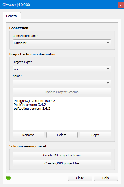
../../../../_images/project-manager.png — Figura 6.1 Giswater project manager window.

As we can see, the window is divided into three parts:

Connection: is the section where we must select the name of the connection with the database we want to use to work. In the case of having several, we can select the desired one in the corresponding dropdown.
Project schema information: this section is formed by three parts. The first, Project type, allows us to select what type of project schema we want to create. The two available options are ws for supply projects and ud for sanitation and urban drainage projects. The second part, Name, indicates the name of the schema. When it appears blank it is because there is no schema created yet. In the case of having several, we can select one or the other in the dropdown. The third and last part is the one formed by a text box in which we will see information related to the created schema. Here we can consult information about the PostgreSQL, PostGis, schema name, EPSG… We also have four buttons available:
- Update schema: button that allows us to update the work schema when we have installed a new version of Giswater, which does not coincide with the creation of the schema. It will only be enabled when the versions do not coincide.
- Rename: button that allows us to rename the schema that we have selected in the Name dropdown.
- Delete: button that allows us to delete the schema that we have selected in the Name dropdown.
- Copy: button that allows us to copy the schema that we have selected in the Name dropdown.
Schema management: section with two buttons which will allow us to create a new schema (Create database project schema) and create the QGIS project (Create QGIS project file).

Once we know the type of project schema to create (ws or ud), we will select it in the Project type dropdown, click on the Create database project schema button and the following window will open.

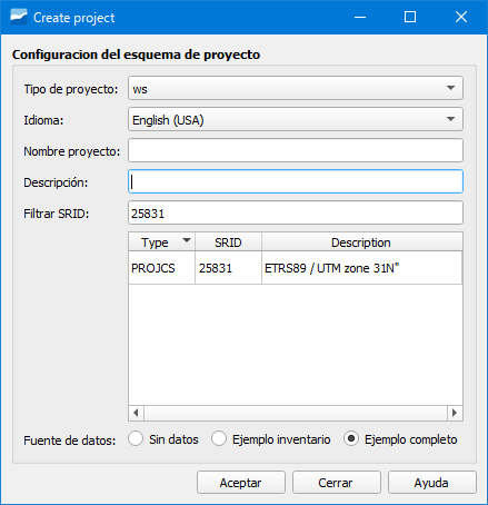
../../../../_images/create-schema.png — Figura 6.2 New schema creation window.

This window serves to specify important aspects of our work schema as well as to create it. We will have to specify:

Project type: type of project we are going to create (ws or ud).
Language: language in which the schema will be created. We can choose one of the available in the dropdown. If we are going to create one of the available examples (Example inventory or Example complete) we will have to select the English (USA) language.
Project name: we will indicate the name of the project schema. It cannot contain uppercase letters.
Description: brief description of the project.
Filter SRID: coordinate system of the zone where the schema will be created.
Data source: we can select between:
- No data: option selected to create a blank schema. It will be the option selected when we want to work with our network.
- Example inventory: option selected to have an example schema only with inventory data.
- Example complete: option selected to have an example schema with complete data (inventory and EPA).

When we have specified all the data, we will click on the Accept button to start the schema creation.

Once the schema has been created, the schema creation window will disappear and we will see that now we have information about the schema in the text box.

Now, the only thing that is left is to create the QGIS project for this we will click on the Create QGIS project file button.

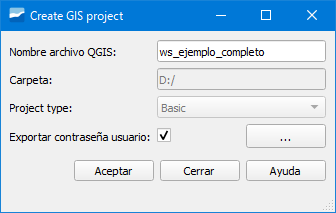
../../../../_images/create-qgis-project.png — Figura 6.3 QGIS project creation window.

In it we will have to specify:

QGIS project name: name we want to give to the project. By default it takes the same name as the schema.
Folder: path where the project will be saved. To be able to change the one that comes we will have to click on the button with three points and a window of the explorer will open.
Export user password: checkbox that allows saving or not the database access password in the GIS file.

When we click on the Accept button the project will be created and opened.

Advertencia

If we mark the Export user password checkbox the password will be saved in the QGIS project. If we share the project with another person we will be sharing our password as well.

Extremar the precaution with the marking of this checkbox.

6.2. Table of contents (ToC)

Once we have the project loaded in QGIS, we see that in the ToC a series of layers have been loaded which are grouped by thematic.

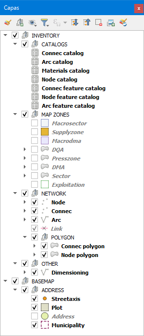
../../../../_images/toc.png — Figura 6.4 Layers of a ws project loaded in the ToC.

INVENTORY group

In this group we are where we find the most important layers of the project since here we find the catalogs (CATALOGS), the map zones (MAP ZONES) and the own layers of the network (NETWORK). There is also an additional group (OTHER) that contains other relevant layers.

BASEMAP group

In this group we find the layers to represent the street axis (Streetaxis), the building polygon (Plot), the portal numbers (Address) and the municipal limit (Municipality).

Giswater incorporates two additional buttons to the ToC of QGIS: Load Giswater layer and Giswater styles.

Load Giswater layer allows us to select which layer we want to add to the project. They are grouped by themes and we can incorporate them by marking the corresponding checkbox. We can also add catalogs and the DEM in the case that we have imported it to the database.

Giswater styles allows us to modify the style of the layers by selecting one of the available ones. As a consequence we will see that the network symbology is modified.

Nota

The styles of the layers can be modified according to the needs of the user. In such a case, to avoid losing the default Giswater symbology, it is recommended to create a new one and not modify the existing one.

6.3. Toolbars 

After opening a Giswater project, we see that we have some toolbars with buttons that allow us to perform different operations. Next, we will see one by one.

6.4. Elements forms 

Each of the network objects defined in the cat_feature_ catalogs has a form associated in which the common fields of the element type are displayed. This is why the forms are quite similar to each other but, as there are also specific fields for each type, there are certain differences.

These forms can be customized so that we can set which fields we want to see, which labels to display and in what color, what position they occupy within the form… As they are unique for each object, the level of customization is such that we can make each form different from the others.

The way to visualize it is through the Info Giswater button and it works for nodes, arcs, connecs, gullys, visits and dimensionings.

6.4.1. Forms parts 

They are formed by three parts or layouts: the upper (1), the central (2) and the lower (3).

Both the upper and the lower will always be visible while the information shown in the middle will be different depending on the object we are consulting and the tab we are visualizing.

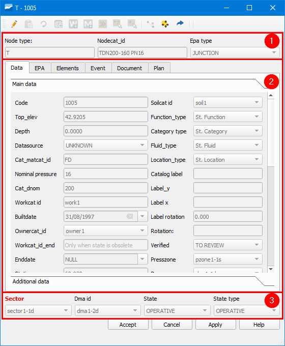
../../../../_images/form.png — Figura 6.15 Example of form of a node of the supply network.

In the upper part we find the widgets that refer to the type of object (Node type) and its specific catalog (Nodecat_id), as well as the EPA type (Epa type).

In the middle part we find the information of each object organized by tabs.

In the lower part we find information about map zones (Sector and Dma id) as well as its state (State) and state type (State type).

Next, using the form of the previous image, we will describe the tabs contained in the middle part.

Nota

Although the form of a network object of the supply network is used as a reference, the tabs of the objects of both types of networks are explained.

Data: contains the data of all the attributes of the object, both the common ones of its type as well as the specific ones of the type of object. It is the most important tab. Depending on the object consulted we will see some data or others.
EPA: refers to the specific data of the EPA world (hydraulic simulation) and will change depending on the EPA type of the element. It consists of two columns. The INP is used to introduce the data necessary for the model and the RPT shows the results of the simulation.
Conections (ud): tab available only for nodes. We will see that there are two parts. The upper part will show all the arcs that are upstream of the node (Upstream features) and the lower part will show all the arcs that are downstream of the node (Downstream features).
Elements: contains information about the associated elements that the object may have. In the case of having associated elements a table with the corresponding data will be seen. Above the table there are several buttons that will allow us to link or unlink existing elements, add new elements or open the data in a floating form.
Relations: tab available only for arcs. We will see a table with the network objects that are connected to the segment (connecs or gullys).
Hydrometer: tab available only for connecs where we will see a table with the list of subscribers associated with the meter.
Hydrometer values: tab available only for connecs that serves to consult the consumptions of the subscribers where we can filter by period and code.
Event: as with the elements, a table with data of the events that have happened over time on our object will be shown. These events refer to all the parameters that have been registered in a visit and we will see information about the date, the type of parameter and its value as well as other data related to the visit. The available buttons allow opening the visit manager, adding a new visit, showing the image related to the event or opening its data in a floating form. In some cases, this tab is replaced by a called Visit which instead of showing the events in table format, shows them in line format having columns for each event.
Document: in it we will see all the documents linked to the object where the most important is the right button, since it allows opening the path and visualizing the selected document.
Plan: refers to the price of the object and will show a list of the costs that the element would have in the case of being renewed. This is especially interesting in the case of arcs, since they have many more variables to consider (soil type, excavation, transport to landfill…). To be able to visualize these prices, the plan_price, cat_soil, cat_pavement catalogs have to be completed and the values of soilcat_id and pavcat_id have to be assigned to the arc layer.